Chapter 4 Best Practices in the Use of Spreadsheets
So you think you know everything about spreadsheets… think again! While probably all of us have used spreadsheets before, it’s easy to misuse them without even knowing you are doing it. This Chapter gives an overview of best practices and common mistakes to avoid.
4.1 What are spreadsheets good for?
Spreadsheets are good tools for data entry. Even though you could technically run some data analyses within your spreadsheet program, that doesn’t mean you should! The main downside to doing data processing and analysis in a spreadsheet is that it entails a lot of pointing and clicking. This makes your analysis difficult to reproduce. If you need to re-run your analysis or re-process some data, you have to do it manually all over again. Also, if you go back to your completed analysis after a while (for example to write the methods of your paper) and you don’t remember what you did, there is no record of it left. This is why this course introduces spreadsheets exclusively as a tool for data entry.
4.2 Human-readable vs. computer-readable data
Most of the problematic practices outlined in this Chapter can be summarized into a single concept: using spreadsheets to convey information in a way that is readable for humans but not for computers. While a human brain is capable of extracting information from context, such as spatial layout, colors, footnotes, etc., a computer is very literal and does not understand any of that. To make good use of spreadsheets, we need to put ourselves in the computer’s mind. All the computer understands from a spreadsheet is the information encoded in rows and columns. So, the number one rule to remember when using spreadsheets is to make your data “tidy”.
4.3 Tidy data
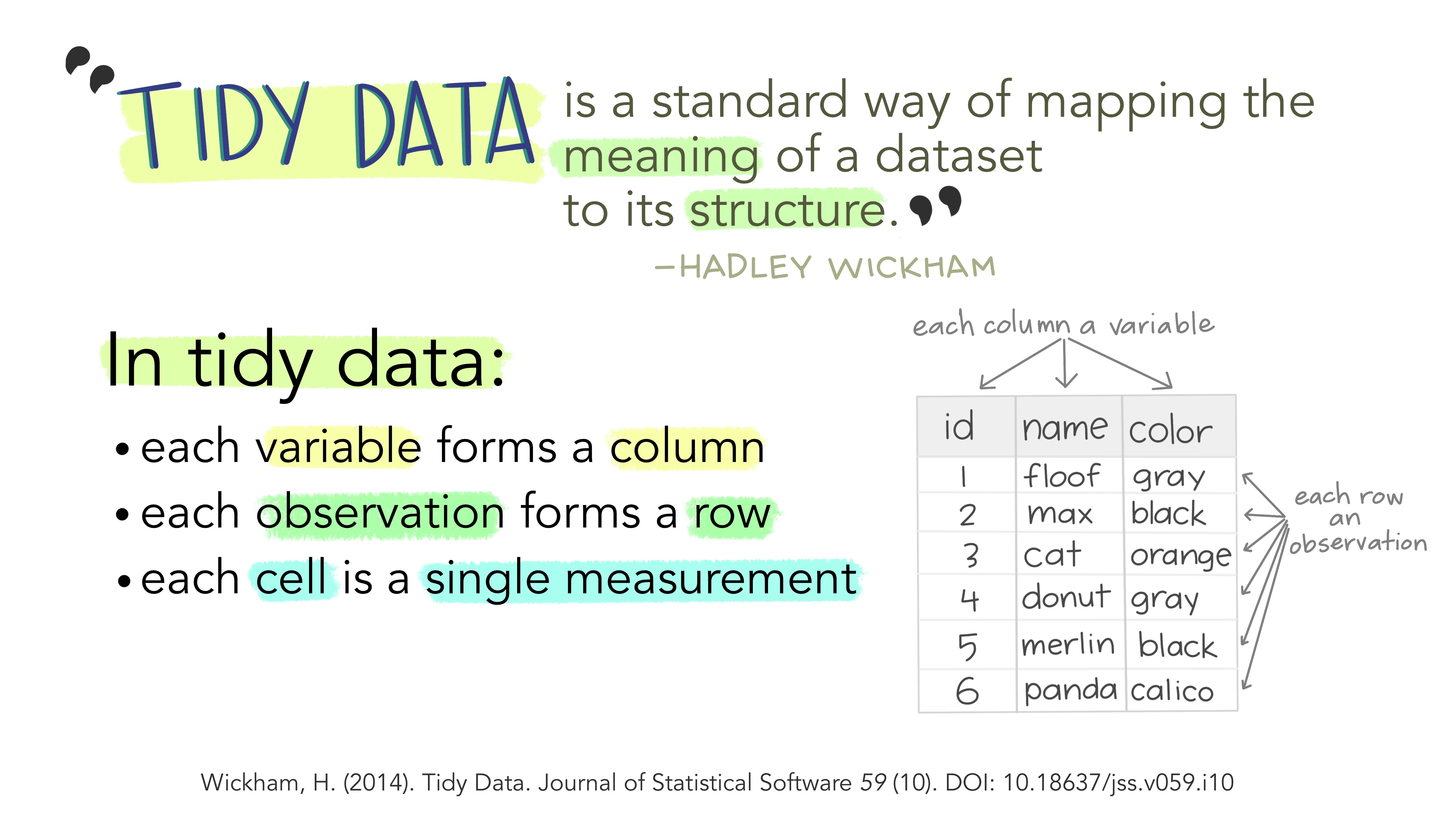
Figure 4.1: Artwork by Allison Horst
The fundamental definition of tidy data is quite simple: one variable per column and one observation per row. Variables are the things we are measuring (e.g., temperature, distance, height.) Observations are repeated measurements of a variable on different experimental units. Structuring your data following this rule will put you in a great position for processing and analyzing your data in an automated way. First, using a standard approach to formatting data, where the structure of a table reflects the meaning of its content (i.e., where a column always means a variable and a row always means an observation) removes any ambiguity for yourself and for the computer. Second, this specific approach works very well with programming languages, like R, that support vector calculations (i.e., calculations on entire columns or tables at a time, instead of single elements only.)
4.4 Problematic practices
In practice, what are some common habits that contradict the principles of tidy data? Here are some examples.
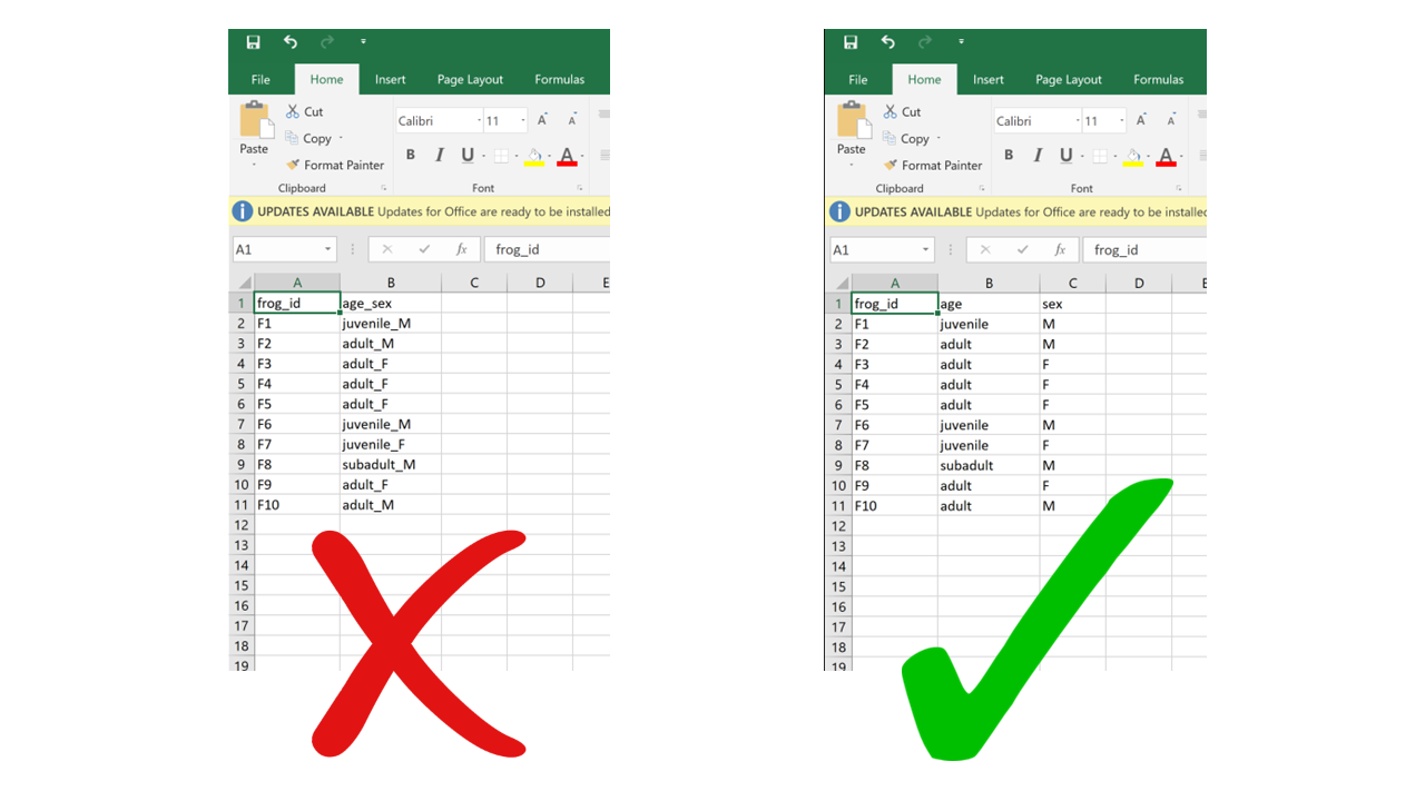
4.4.1 Multiple variables in a single column
Putting information for two separate variables into one column contradicts the “one column per variable” principle. A classic example of this is merging age class and sex into one – for example “adult female”, “juvenile male”, etc. If, for instance, later on we wanted to filter based on age only, we would have to first separate the information within the column and then apply a filter. It is much more straightforward to combine information than to split it, so the structure of our data should always follow a reductionist approach where each table unit (cell) contains a single data unit (value).
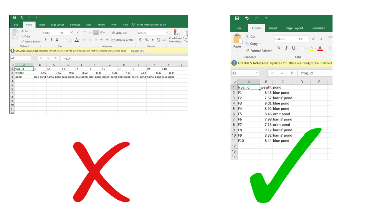
4.4.2 Rows for variables, columns for observation
While the choice of using rows for observations and columns for variables may seem arbitrary – after all, why can’t it be the other way around? – consider this: the most commonly used data structure in R, the data frame, is a collection of vectors stored as columns. A property of vectors is that they contain data of a single type (for instance, you can’t have both numbers and characters in the same vector, they either have to be all numbers or all characters). Now imagine a situation where a dataset includes weight measurements of individual green frogs captured in different ponds: for each frog, we’d have a weight value (a number) and the name of the pond where it was captured (a character string). If each frog gets a row, we get a column for weight (all numbers) and a column for pond (all characters). If each frog gets a column and weight and pond go in different rows, each column would contain a number and a character, which is not compatible with R. This is valid not only for R, but for other vector-based programming languages too. The tidy data format makes sure your data integrates well with your analysis software which means less work for you getting the data cleaned and ready.
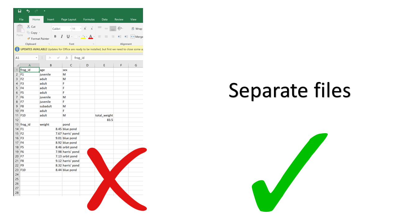
4.4.3 Multiple tables in a single spreadsheet
Creating multiple tables in a single spreadsheet is problematic because, while a human can see the layout (empty cells to visually separate different tables, borders, etc.) and interpret the tables as separate, the computer doesn’t have eyes and won’t understand that these are separate. Two values on the same row will be interpreted as belonging to the same experimental unit. Having multiple tables within a single spreadsheet draws false associations between values in the data. Starting from this format will invariably require some manual steps to get the data into a format the computer will read. Not good for reproducibility!
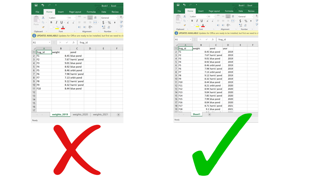
4.4.4 Multiple sheets
This one may seem innocuous, but actually it can be problematic as well. For starters, you can’t load multiple sheets into R at the same time (by multiple sheets, I mean the tabs at the bottom). If you’re only using base R functions, you can’t even load a .xslx file (although you can using packages such as readxl), so you’re going to have to save your spreadsheets as .csv before importing. When saving as .csv, you’ll only be able to save one sheet at a time. If you’re not aware of this, you end up losing track of the data that was in the other sheets. Even if you are aware, it just makes it more work for you to save each of the sheets separately.
Using multiple sheets becomes even more of a problem when you are saving the same type of information into separate sheets, like for example the same type of data collected during different surveys or years. This contradicts another principle of tidy data, which is each type of observational unit forms a table. There’s no reason to split a table into multiple ones if they all contain the same type of observational unit (e.g., morphometric measurements of frogs from different ponds). Instead, you can just add an extra column for the survey number or year. This way you avoid inadvertently introducing inconsistencies in format when entering data, and you save yourself the work of having to merge multiple sheets into one when you start processing and analyzing.
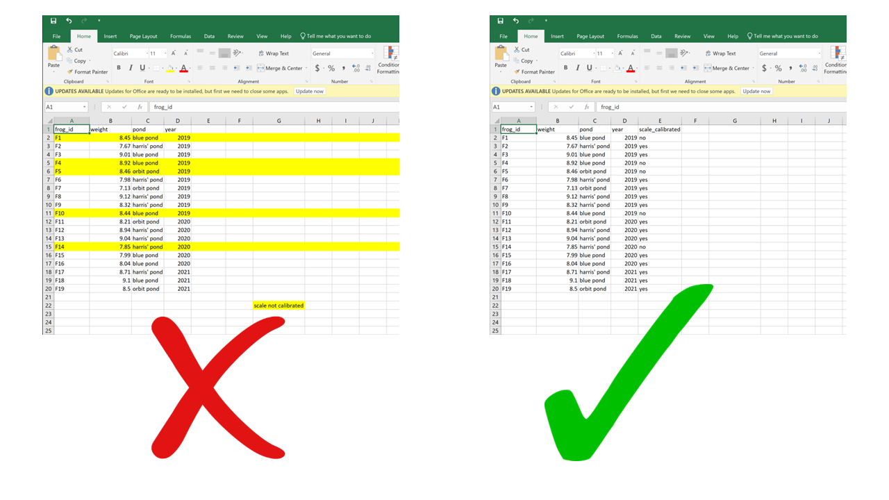
4.4.5 Using formatting to convey information
Anything that has to do with visual formatting is not computer-readable. This includes borders, merging cells, colors, etc. When you load the data into an analysis software, all the graphical features are lost and all that is left is… rows and columns. Resisting the temptation to merge cells, and instead repeating the value across all rows/columns that it applies to, is making your data computer-friendly. Resisting the urge to color-code your data, and instead adding an additional column to encode the information you want to convey with the different colors, is making your data computer-friendly. Columns are cheap and there’s no such thing as too many of them.
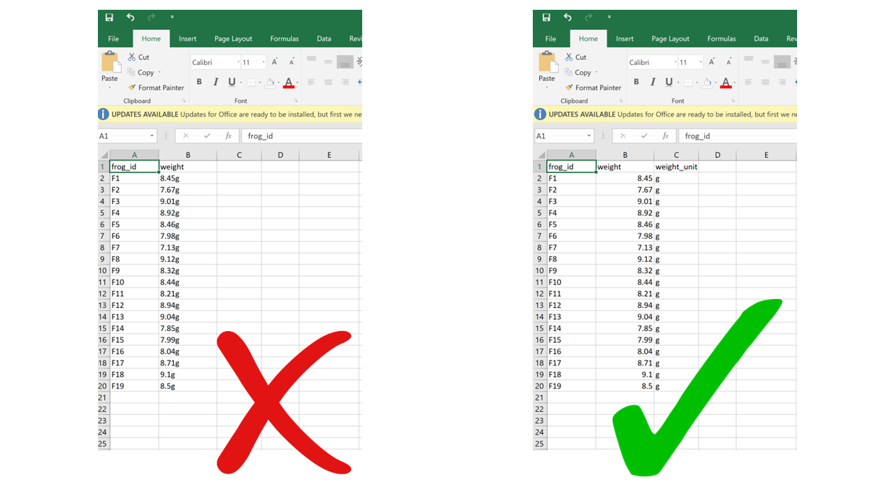
4.4.6 Putting units in cells
Ideally, each measurement of a variable should be recorded in the same units. In this case, you can add the unit to the column name. But even if a column includes measurements in different units, these units should never go after the values in the cells. Adding units will make your processing/analysis software read that column as a character rather than as a numeric variable. Instead, if you need to specify which unit each measurement was taken in, add a new column called “variable_unit” and report it there. Remember, columns are cheap!
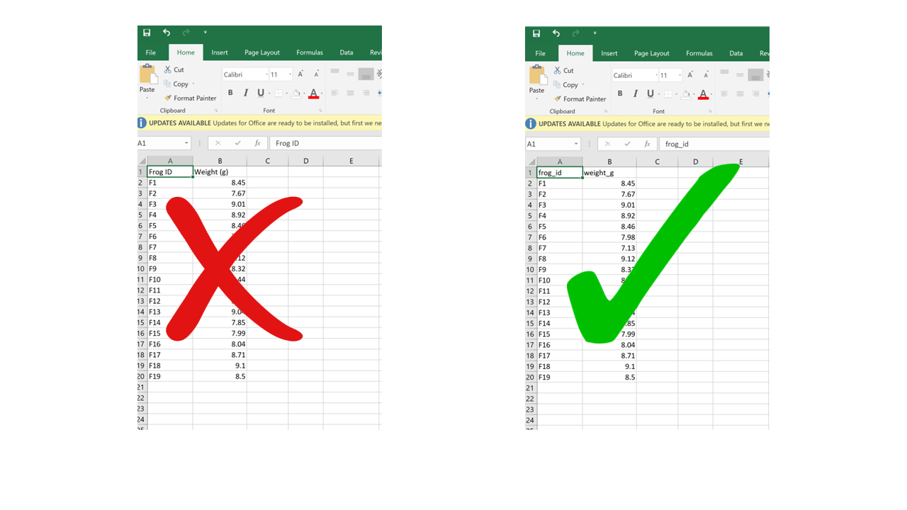
4.4.7 Using problematic column names
Problematic column names are a lot like the problematic file names from Chapter 1. They are non-descriptive, they contain spaces or special characters – in short, they are human-readable but not computer-readable. Whether you separate words in column names using camel case or underscores, avoid using spaces. It’s a good idea to include units in the column names, e.g., “weight_g”, “distance_km”, etc. Also, just like for file names, be consistent in your capitalization pattern and choice of delimiters.
4.4.8 Conflating zeros and missing values
Conflating zero measurements with missing values by using a zero or a blank cell as interchangeable is a problem, because there’s a big difference between something you didn’t measure and something that you did measure and it was zero. Any blank cell will be interpreted as missing data by your processing/analysis software, so if something is zero it needs to be actually entered as a zero, not just left blank. Similarly, never use zero as your value for missing data. These are two separate meanings that need to be encoded with different values.
4.4.9 Using problematic null values
Many common ways to encode missing values are problematic because processing/analysis software does not interpret them correctly. For example, “999” or “-999” is a common choice to signify missing values. However, computers are very literal, and those are numbers. You may end up accidentally including those numbers in your calculations without realizing because your software did not recognize them as missing values. Similarly, like we said, “0” is indistinguishable from a true zero and should never be used to signify “missing data”. Worded options, such as “Unknown”, “Missing”, or “No data” should be avoided because including a character value into a column that is otherwise numeric will cause the entire column to be read as character by R, and you won’t be able to do math on the numbers. Using the native missing value encoding from your most used programming language (e.g., NA for R, NULL for SQL, etc.) is a good option, although it can also be interpreted as text in some instances. The recommended way to go is to simply leave missing values blank. The downside to this is that, while you’re entering data, it can be tricky to remember which cells you left blank because the data is missing and which ones are blank because you haven’t filled them yet. Also, if you accidentally enter a space in an empty cell, it will look like it’s blank when it actually is not.
4.4.9.1 Inconsistent value formatting
A very common problem arises when having to filter/tally/organize data based on a criterion that was recorded inconsistently in the data. I find this to be especially common for columns containing character-type variables. For example, if the person entering data used “F” or “Female” or “f” interchangeably in the “sex” column, it will be difficult later on to know how many female individuals are in the dataset. Similarly, if the column “observer” contains the name of the same person written in multiple different ways (e.g., “Mary Brown”, “Mary Jean Brown”, “M. Brown”, “MJ Brown”), these won’t be recognized as the same person unless these inconsistencies are fixed later on.
4.5 Document, document, document!
If you follow all the guidelines outlined in this Chapter, chances are you will be able to automate all of your data processing without having to do anything manually, because the data will be in a computer-readable format to begin with. However, if you do end up having to do some manual processing, make sure you thoroughly document every step. Like we discussed in Chapter 1, never edit your raw data; save processed/cleaned versions as new files; and describe all the steps you took to get from the raw data to the clean data in your README file.
4.6 References
- https://datacarpentry.org/spreadsheet-ecology-lesson
- Wickham, Hadley. “Tidy data.” Journal of Statistical Software 59.10 (2014): 1-23.
- White, Ethan P., et al. “Nine simple ways to make it easier to (re) use your data.” Ideas in Ecology and Evolution 6.2 (2013).