Chapter 10 Introduction to R
10.1 Getting started
Some of you may already be familiar with R, so we are going to go over some basics and then breeze through the fundamentals of R programming to get to the more advanced stuff.

Figure 10.1: Artwork by Allison Horst
Let’s start with some definitions: R is both a programming language and a software. However, the R software is just an R command line and it has no additional interface. RStudio is an Integrated Development Environment (IDE) that facilitates working with R by providing an interface that makes it easy to save code script, keeping track of your working environment, looking up your directory structure, and visualize your plots while you’re coding. We’ll be using RStudio throughout the remainder of this course. Remember what we said in Chapter 1 about RStudio Projects – make sure you are always working within a Project and you’re aware of your working directory!
You can check what Project you are working on on the top-right corner of your RStudio window. When you open up a Project, the working directory will show up in the Files tab in the bottom-right panel. This is also the panel where your plots appear and where you can look up help files for R functions. The top-left panel is where you will type your code to then save it in a script. The bottom-left panel is the console and it is where you will see results and run any line of code that you do not need to save. The top-right panel has several tabs but by default it shows your R environment, that is, all the objects and functions that exist in your session at any given time.
When you want to run code from your script, you can send it to the console to execute by pressing Ctrl (or Cmd) + Enter. If nothing in the script is highlighted, the command that gets run is the one where your cursor is. If something is highlighted, that will be the only piece of code that gets run (this will turn out to be very useful).
The > prompt means R is ready to execute a command. If a + sign shows up
instead, it means the code you tried to run is incomplete (in many cases,
this means you’re missing a closing parenthesis). You can press Esc to abort the
command when this happens and you’re not sure what’s missing.
10.2 Basics of R programming
10.2.1 Assigning objects
The <- operator is called an assignment operator. Whatever is on the right of
the arrow is going to be assigned to the name on the left, and the object will
show up in your Environment tab on the top-right. A shortcut for the assignment
operator is Alt + -.
You can name an object anything you want, but the name cannot start with a number. Also, R is case-sensitive, so make sure you are consistent with uppercase/lowercase. Back in the day someone would have told you to choose names that are short so you save yourself some typing, but RStudio has an autocomplete option that makes this not a problem at all, so I say: above all, choose names that are descriptive because that will make your code much more readable and easy to understand!
10.2.2 Adding comments
One of the recommendations you are going to hear most often is, “always comment
your code”. Indeed, it is very important to make sure your scripts contain
enough information that a reader unfamiliar with your code (a colleague, or
yourself in a few weeks) can understand what’s going on and what each piece is
doing. You can add comments using a hashtag. Anything on a line after the #
will not be treated as code.
10.2.3 Headers and description
Even when I’m not writing an RMarkdown file and I’m just working with a .R file, I like to start my scripts with a header that says who the author is, what the script is about, when it was created, and when it was last modified. Something like this:
# # # # # # # # # # #
# Simona Picardi
# Getting started with R
# Created January 8th, 2020
# Last modified January 25th, 2020
# # # # # # # # # # #
After the header, I like to add a general description providing some context of what the script does and where it fits in with related ones. For example, you may want to describe what project the script is part of, what is it for, what are the inputs and outputs, etc.
10.2.4 Navigating through the script
Often you’ll find yourself writing scripts that are many many lines long. If you are looking for a specific piece within a large script, you could spend a long time crossing your eyes trying to find it. Because nobody likes their eyes to bleed, it’s much more convenient to add bookmarks to your script so that you can easily jump to the section you’re looking for. You can add a bookmark using four hastags like so:
The Data processing and Data analysis bookmarks will appear under your script panel and you can click to navigate between them.
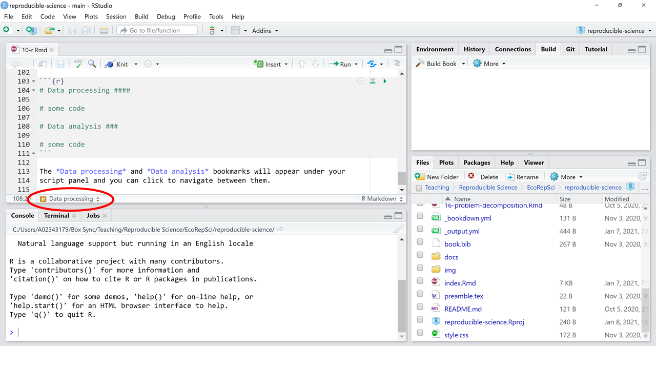
Figure 10.2: Bookmarks in RStudio help you efficiently navigate your script
10.2.5 Functions and their arguments
A function is an executable scripts that takes a well-defined input and returns
a certain desired output. The inputs of a function are called arguments. For
example, the function round takes as input an argument called x which is
the number you want to round:
## [1] 10The function takes also a digits argument, although it is optional: if we
don’t specify it will just use the default value. You can check what the default
is by looking at the help file for the function:
The default is 0 decimal digits, so unless we specify something different the
function will round to the closest integer. Arguments that are optional are also called options. It’s important to be aware of what default values are assigned
to optional arguments when we don’t manually specify them. Another thing to be
aware of is that function interpret their inputs positionally unless the
arguments are explicitly spelled out. So for example, running round(10.465, 1)
is the same as running round(x = 10.465, digits = 1). If we shuffle the order
of the inputs and do round(1, 10.465) the function won’t understand that x is
10.465 and not 1. But if we spell out which input is which, the order no longer
matters: round(digits = 1, x = 10.465) works just fine.
10.2.6 Writing functions
Now that we learned about the anatomy of a function, we can write our own. A
function is like a recipe where the arguments are the ingredients and the
function code is the procedure. At the end, you get your baked goods. The
syntax to write a function is function(arguments){code}. First, we define what
inputs the function should take (i.e., we pick names for the arguments). Then,
inside the curly braces, we describe what the function does with those inputs.
For example, let’s write a function to add two numbers together:
# We'll call this function 'add'.
add <- function(x, y) { # It takes as input two arguments named `x` and `y`
  return(x + y) # and it returns x + y
}

add(4, 5)
## [1] 9We can then assign this value to an object:
(z <- add(4, 5)) # by wrapping the assignment statement in parentheses I also automatically print it to the console## [1] 9We can also write functions that, instead of returning a value that can be assigned to an object, print something in the console without returning anything:
## [1] "Hello world!"## [1] "Hello Simona!"10.2.7 Data types
Data in R can be of several types. The four most common ones are character,
numeric, integer, and logical. There’s also complex and raw, but we
won’t talk about those here. Character data consists of strings of text and it
is defined using quotes:
## [1] "character"Numbers and integers are pretty self-explanatory. Logical data is boolean TRUE/
FALSE:
## [1] "logical"10.2.8 Vectors
A vector (or atomic vector) is the most basic data structure in R. It is a
collection of items of the same data type. You can concatenate different elements
into a vector using c:
## [1] "numeric"## [1] "character"As a matter of fact, a vector that only has one element is still a vector! So
x <- 43 is a vector with 1 element (that is, a vector of length = 1).
You can’t have elements of different data types within the same vector. If we try to mix data types inside a vector, R will fall back to the data type that is most inclusive and interpret all the elements in the vector as belonging to that data type. For example, if we do:
## [1] "character"R interpreted the whole vector as character because there’s no way to turn “B” into a number, but you can read numbers as text strings. If instead we do:
## [1] "numeric"R interprets the whole vector as numeric because TRUE and FALSE are encoded
as 1 and 0, respectively. So R converted the logical element into a number and
now the entire vector is numeric. If we mix logical and character, character
will win because there is no way to turn a text string into TRUE or FALSE,
but TRUE and FALSE are literally words so it’s easy to read them as text:
## [1] "character"Anything in quotes is always interpreted as character, no matter what:
## [1] "character"## [1] "character"So, in the hierarchy of data types, character is the most general because you
can always turn something into a character; numeric follows because you can
read all other data types (integer and logical) as numbers; and logical is
the least general because you cannot turn any of the others into logical. The
process of converting an object of one type into another type is called
coercing. You may run into this term in error messages so it’s good to know
what it means so you can diagnose problems.
10.2.9 Factors
Categorical data is represented in R using factors. A factor is stored as a vector of labels called levels but, under the hood, each level gets assigned an integer (or index value). R uses the integer component of a factor to do its job but it displays the level to you so that it’s descriptive and meaningful. This weird nature of factors is often a source of confusion. For example, if we have the following factor,
and we want to convert the years back into numeric, we would maybe try:
## [1] 1 2 3 4 5The result is not what we expected. This is because R converted the index values into numbers, not the factor levels. To specify that we want to convert the factor levels into numbers, not the underlying vector of integers, we have to be explicit about it:
## [1] 2017 2018 2019 2020 202110.2.10 Data frames
R stores tabular data in data frames. A data frame is a data structure composed by rows and columns, where each column is a vector (and therefore contains elements of the same type). Different columns in a data frame can contain data of different type but they must all be the same length or they won’t line up. More often than not, you’ll create data frames by importing external files (such as .csv) or by connecting to a SQL database, in which case the output of a query is returned as a data frame by RSQLite (see Chapter 7). But you can also manually create a data frame:
df <- data.frame(numbers = c(1, 2, 3),
                 letters = c("A", "B", "C"),
                 colors = factor(c("blue", "red", "green")))

str(df)
## 'data.frame': 3 obs. of 3 variables:
## $ numbers: num 1 2 3
## $ letters: chr "A" "B" "C"
## $ colors : Factor w/ 3 levels "blue","green",..: 1 3 2Using str to look at the structure of the data frame, we can confirm that it
contains three columns: a numeric vector, a character vector, and a factor.
You can select columns of a data frame by name using a $:
## [1] blue  red   green
## Levels: blue green red
10.2.11 Dimensions
One thing that it’s important to be aware of is the dimensions of the objects we work with. A vector is a one-dimensional data structure. If we wanted to make an analogy with geometry, a vector is like a line. There is no scalar in R because a single element is still a vector (of length 1). A data frame is like a plane because it has two dimensions (rows and columns). This is important to understand because it determines how we subset data. For example, let’s look at the dimensions of the data frame we just created:
## [1] 3 3This is a 3x3 object (3 rows and 3 columns), and therefore it has 2 dimensions. A vector, on the other hand, only has a length (its one dimension):
## [1] 2Matrices are also 2-dimensional objects like data frames, but they differ from data frames because they can only contain elements of the same data types, while columns in a data frame can be of different data types. For example:
##      [,1] [,2] [,3] [,4] [,5]
## [1,]    1    6   11   16   21
## [2,]    2    7   12   17   22
## [3,]    3    8   13   18   23
## [4,]    4    9   14   19   24
## [5,]    5   10   15   20   25
Arrays are objects that can have more than 2 dimensions. For example, an array with 3 dimension is like a 3D matrix, where the first dimension is the number of rows, the second is the number of columns, and the third is the number of matrices that compose the array. For example:
## , , 1
##
##      [,1] [,2] [,3] [,4]
## [1,]    1    3    5    7
## [2,]    2    4    6    8
##
## , , 2
##
##      [,1] [,2] [,3] [,4]
## [1,]    9   11   13   15
## [2,]   10   12   14   16
##
## , , 3
##
##      [,1] [,2] [,3] [,4]
## [1,]   17   19   21   23
## [2,]   18   20   22   24
This array has 3 dimensions:
## [1] 2 4 310.2.12 Subsetting
Knowing how many dimensions an object has makes it straightforward to write syntax to subset it. For example, to subset the following vector to only include the first two elements:
We can specify which elements we want to subset in brackets:
## [1] "blue" "red"# A better way to write this:
test[1:2] # using : automatically returns a vector of integers from the number on the left to the one on the right## [1] "blue" "red"The numbers in square brackets provide the indexes of the elements we want to keep. For an object that has more than one dimension, we need to specify 2 sets of indexes, one for each dimension. In the case of a data frame, these would be rows and columns:
##   numbers letters colors
## 1       1       A   blue
## 2       2       B    red
## 3 3 C green## [1] "A"## numbers letters colors
## 1 1 A blue## [1] "A" "B" "C"Note that when we subset a column, the output is a vector (all elements are of the same type). But when we subset a row, the output is still a data frame (elements need not be of the same type):
## [1] "character"## [1] "data.frame"If you want to exclude a row or a column instead of keeping it, you can use a -
in front of the index:
## letters colors
## 1 A blue
## 2 B red
## 3 C green## numbers letters colors
## 1 1 A blue
## 3 3 C greenWe can subset a matrix with positional indexes the same way we would subset a data frame:
## [1] 6To subset rows, columns, or matrices within a 3-dimensional array we need to use 3 indexes instead of 2, like we’ve been doing for matrices and data frames. For example, to subset the first row:
## [,1] [,2] [,3]
## [1,] 1 9 17
## [2,] 3 11 19
## [3,] 5 13 21
## [4,] 7 15 23To subset the first column:
## [,1] [,2] [,3]
## [1,] 1 9 17
## [2,] 2 10 18To subset the first matrix:
## [,1] [,2] [,3] [,4]
## [1,] 1 3 5 7
## [2,] 2 4 6 810.2.13 Logical conditions
Logical conditions are statements that can be answered with TRUE or FALSE.
For example, is 10 greater than 5?
## [1] TRUEIs 2 + 2 = 3?
## [1] FALSEIs df a data frame?
## [1] TRUELogical conditions are very useful for conditional subsetting. More often than wanting to subset a specific row or column of a data frame, we may want to subset rows based on a condition. For example, if we only want rows where the color is blue:
##   numbers letters colors
## 1 1 A blueInstead of putting a numeric index where we tell R which rows we want, we used a logical condition. R will evaluate that logical condition and only keep the rows for which it’s true. Let’s decompose that:
## [1] TRUE FALSE FALSEWhen you plug in the above statement in place of the subsetting index, R will
return the rows that satisfy the condition (the ones that return TRUE):
##   numbers letters colors
## 1 1 A blueNote that a double equal == will evaluate a logical condition, while a single
equal sign = is equivalent to an assignment operator <-. These are not the
same thing!
To exclude a column or a row when using conditional subsetting, we can’t use -
like we did when we were using indexes. Instead, logical conditions are denied
with !:
## numbers letters colors
## 2 2 B red
## 3 3 C greenIn the example above, we write the logical condition “color is equal to blue”
and then we deny it by putting ! in front of it. We can also directly write
the logical condition “color is NOT equal to blue”:
## numbers letters colors
## 2 2 B red
## 3 3 C greenSo far, we have seen four logical operators: >, <, ==, !=. Another one
you’ll be finding yourself using a lot is %in%, which tests whether a value is
within a list of values:
##   numbers letters colors
## 1       1       A   blue
## 2 2 B red10.2.14 Lists
Lists are the most flexible data structure in R. They can contain elements of different data type and size. For example:
## [[1]]
## [1] 1
##
## [[2]]
## [1] 1 2
##
## [[3]]
##  [1]  1  2  3  4  5  6  7  8  9 10
# This list contains vectors of different data types
(list2 <- list(1:5, c("cat", "dog", "lion", "giraffe")))## [[1]]
## [1] 1 2 3 4 5
##
## [[2]]
## [1] "cat" "dog" "lion" "giraffe"# This list contains a numeric vector, a character vector, a matrix, and a function
(list3 <- list(1:10, c("A", "B"), matrix(0, 4, 4), function(x) {x + 1}))## [[1]]
## [1] 1 2 3 4 5 6 7 8 9 10
##
## [[2]]
## [1] "A" "B"
##
## [[3]]
## [,1] [,2] [,3] [,4]
## [1,] 0 0 0 0
## [2,] 0 0 0 0
## [3,] 0 0 0 0
## [4,] 0 0 0 0
##
## [[4]]
## function(x) {x + 1}We can name the elements of a list:
## $numbers
##  [1]  1  2  3  4  5  6  7  8  9 10
##
## $letters
## [1] "A" "B"
##
## $matrix
##      [,1] [,2] [,3] [,4]
## [1,]    0    0    0    0
## [2,]    0    0    0    0
## [3,]    0    0    0    0
## [4,]    0    0    0    0
##
## $`function`
## function(x) {x + 1}
We can subset lists by using double brackets. For example, to extract the second
element of list3 we would do:
## [1] "A" "B"This returns the character vector with the letters A and B. Using a single bracket instead of a double bracket will return a list with the element/s we called for:
## $letters
## [1] "A" "B"
Imagine the single bracket as returning the bin where the object is and the double bracket as returning the actual content of the bin.
10.2.15 Control structures
Control structures allow you to “activate” or “de-activate” your code based on circumstances you can define as you need. Think of them as switches that modulate the operations you do on your data.
The most commonly used control structure in R is the combination of if and
else. By using if, you can specify a logical condition and the code that you
want to run if that condition is verified. The syntax is as follows:
If condition returns TRUE, the code in the curly braces will be executed,
otherwise it won’t. If you want to specify what to do in case the condition is
FALSE, you can pair the if with an else:
Other control structures include break, which stops a loop when a condition
is met, and next, which skips one iteration of a loop. Loops themselves are
control structures, but we’ll talk about them in the next section.
10.2.16 Repeating operations
Many times in R you will find yourself having to repeat the same operation over
a set of values/rows. There are multiple ways to do so: vectorized operations,
loops, and apply functions.
10.2.16.1 Vectorization
Unlike many other programming languages, R supports vectorization, which means some operations can be carried out in parallel across R objects. Without knowing, we’ve already made some examples of vectorized calculations in R. For instance, applying a logical comparison to all elements of a vector:
## [1] FALSE FALSE FALSE FALSE TRUE TRUE TRUE TRUE TRUE TRUEThe sum of two vectors can also be vectorized:
## [1] 7 9 11 13 15In languages that don’t use vectorization, you would have to write a loop to
sum each element of x to the corresponding element of y. Vectorization makes
many operations very fast and it also makes your code more readable because all
you have to type is x + y instead of for (i in 1:length(x)) {for (j in 1:length(y)) {sum(x[i], y[j])}}…
A pitfall that it’s important to be aware of when doing vectorized calculations
is vector recycling. In the example above, the two vectors x and y have the
same length: they are each composed of five elements. If we try to do a
vectorized calculation on two vectors that aren’t the same length, R will
recycle values from the shortest vector when it runs out, leading to unexpected
results:
## Warning in x + y: longer object length is not a multiple of shorter object
## length
## [1] 8 10 12 14 12 14The vector y has only 4 elements. So for the first 4 values we got what we
expected: 1 + 7, 2 + 8, 3 + 9, 4 + 10. From the fifth value onwards, R kept
going with the values of x but started over with y and returned 5 + 7,
6 + 8. The output was accompanied by a warning message. Whenever you see this
warning message, it means there’s an instance of vector recycling going on in
your code.
10.2.16.2 Loops
The first thing to know about loops is when you should or shouldn’t use a loop. Loops can be inefficient when compared to vectorized alternatives, so whenever you can do what you need by using a vectorized operation, do that instead of a loop.
The second thing to know about loops is that there are multiple types of them
(for, while, repeat). These mostly differ in the way you tell the loop how
many times it should repeat the operation. Most of the time you’ll find yourself
using for loops, so we’ll go over those in detail.
A for loop is written by specifying how many times we want to repeat an
operation and what is the operation we want to repeat:
This can be as simple as printing the numbers from 1 to 10:
## [1] 1
## [1] 2
## [1] 3
## [1] 4
## [1] 5
## [1] 6
## [1] 7
## [1] 8
## [1] 9
## [1] 10
Or it can be more complicated, such as multiple consecutive operations:
## [1] 6
## [1] 20
## [1] 42
## [1] 72
## [1] 110
## [1] 156
## [1] 210
## [1] 272
## [1] 342
## [1] 420
The two examples above print the results to the console. If you want to store the results, you start by defining an object that will store the values as you compute them:
10.2.16.3 The apply family
Functions from the apply family include apply, sapply, tapply, mapply,
vapply, lapply. All of these functions work similarly to a loop by applying
the same operation to a certain piece of input data. However, they differ from
one another in the data structure they take in input and those they return in
output.
The most basic member of the family is the apply function. This takes as input
a matrix or array and it can return a vector, an array, or a list according to
what we’re asking it to do. The function takes three arguments:
Xis the matrix or array that we’re doing calculations on;MARGINspecifies whether we want to apply the operation across rows (if set to 1) or columns (if set to 2);FUNis the function we want to apply.
For example, remember our matrix?
##      [,1] [,2] [,3] [,4] [,5]
## [1,]    1    6   11   16   21
## [2,]    2    7   12   17   22
## [3,]    3    8   13   18   23
## [4,]    4    9   14   19   24
## [5,]    5   10   15   20   25
We can use apply to get a row-wise sum:
## [1] 55 60 65 70 75All other members of the apply family are a variation on this basic theme.
One other member of the apply family that you will find extremely useful is
lapply. This function applies an operation to each element of a list. Given
the flexibility lists give in terms of what they can contain, using lapply
opens up a world of possibilities in terms of what kind of operations we can
automate. Here is a basic example that illustrates how to use lapply:
## [[1]]
##  [1]  1  2  3  4  5  6  7  8  9 10
##
## [[2]]
##  [1]  2  3  4  5  6  7  8  9 10 11 12 13 14 15 16 17 18 19 20
##
## [[3]]
##  [1]  3  4  5  6  7  8  9 10 11 12 13 14 15 16 17 18 19 20 21 22 23 24 25 26 27
## [26] 28 29 30
Notice that this list contains 3 elements of different length. This means they
could not be rows or columns in the same matrix or data frame, and we couldn’t
just use apply to repeat an operation on each of them. But because we’re using
a list and lapply, we can. If we want to get the sum of values within each
element of the list:
## [[1]]
## [1] 55
##
## [[2]]
## [1] 209
##
## [[3]]
## [1] 462
Or if we want to apply a custom function:
## [[1]]
## [1] 917.5
##
## [[2]]
## [1] 923
##
## [[3]]
## [1] 928.5