Chapter 5 Relational Databases

5.1 What is a relational database?

A relational database is a collection of interrelated tables. The relationships between tables represent actual relationships between data entities. The relationships between data entities always exist in real life, no matter our choice of data management system; but they are only made explicit to the computer when the data are stored in a relational database.

For example, say that we collected data in the field for green frogs where, the first time an individual is captured, we record its sex, take some biometric measurements, and assign it an ID. Then, the animals are recaptured periodically to take new biometric measurements. We’d store our data in two spreadsheets, one that has a list of all the frogs we’ve ever captured with their ID and sex. The second spreadsheet has all the biometric measurements, and each frog ID may appear more than once. The two spreadsheets are related because they both contain information about the same individuals: the first one contains one-time information, and the second one contains repeated records for each individual. However, the computer does not know about this relationship, only we do. By using a relational database we translate real-world relationships between data entities into structural relationships between our data tables.

5.2 Why bothering with relational databases?

You may ask, why should we care to enforce structural relationships between tables? Isn’t it enough to just know how things are related? Well, the first advantage of relational databases is that they force us to think critically about the real-life relationships between data entities, which we often take for granted and we might overlook. Many problems with data inconsistencies directly stem from not having a robust logical structure to our data organization.

Enforcing a logical data structure goes hand in hand with quality control and assurance. By designing a mental map of what the different pieces of information look like and how they relate to one another, we can easily spot conditions that need to be verified in order for the data to make sense. If any of those conditions aren’t verified, something isn’t right. For example, imagine having a table of capture and mortality dates for the frogs in addition to biometric measurements. It is logically impossible for any of the biometrics measurements of an individual to be taken outside of the interval between first capture and death. If we store our data in spreadsheets, we may not even notice if there’s a record supposedly taken before an individual was captured or after it died. But if we make the relationship between the two tables explicit, the computer will recognize impossible situations like these for us.

Another advantage of relational databases is that they allow for optimal data storage by avoiding redundancy of information across tables. There is no need to repeat the same data across multiple tables because the relationships between tables allow us to cross-link data across them. For example, there is no need to repeat the sex and capture date of an individual frog for each biometrics measurement we take of that individual. As long as we can relate the two tables based on the individual ID, we can always retrieve and combine information across them. This improves accuracy by avoiding duplication and it reduces the space our data occupies on our computer.

There are several more advantages to using relational databases, including fast (like, extremely fast) processing over large amounts of data. If the database is stored on an external server, that also helps managing data across collaborators within a project by having a centralized repository that everybody can connect to and use, which means everyone always has the same and most up-to-date version of the data. It’s also possible to set up user profiles with different privileges, like read-and-write or read-only. Storing the database on an external server also means that data processing and computation don’t happen on your local computer and thus they don’t take up your memory, which is often limited. Finally, concepts of relational database management are key to understanding data manipulation in other languages.

5.3 Database components

The core unit of a relational database is a table: a two-dimensional structure composed by rows (or records), and columns (or fields). Each row is an observation and each column is a variable (sounds familiar? We talked about tidy data in 4.3)

Tables relate to one another through foreign keys. A foreign key is a variable that is shared between two tables. For instance, in the frogs example above, the individual ID is the variable relating each biometric measurement to the static features of each individual (sex, first capture date, mortality date.) Foreign keys are what makes relational databases “relational”. A table can have one or more foreign keys, each relating it to another table.

In addition to foreign keys, each table in a relational database also has a primary key. A primary key is a unique identifier for each record in the table. Sometimes one variable lends itself well to being a primary key, for example the individual ID would be a suitable primary key for the table of static individual information, because each individual appears only once and thus the ID is a unique identifier of rows. However, the individual ID would not be a suitable primary key for the table of biometric measurements, because IDs are repeated and therefore not unique. When there isn’t a suitable variable to serve as a primary key, we can simply add a serial number that uniquely identifies each record.

5.4 Database design and architecture

The structure of a database should reflect real-world structure in the data. The way we split data into tables and the relationships we enforce between them should mirror the real way data entities relate to one another. Designing a database has little to do with software and coding and everything to do with thinking about the real structure in our data and how can we best represent it using the building blocks of a database.

In general, tables should we split based on the sampling unit of the data they contain. For example, data on individual frogs and data on the ponds where the frogs came from should be stored in separate tables. One table has the frog as its unit and one has the pond. These two tables could then be put in relation based on the pond each frog was caught in.

Two tables may still deserve to be split even if they refer to the same real-world sampling unit. The example we made at the beginning where we have a table of individual ID and sex and a table of individual biometric measurements is a good illustration for this. In both of those tables, the sampling unit is an individual frog, but the first table contains static information that does not change through time, whereas the second table contains dynamic information, which translates into repeated measures for each individual. Instead of keeping these data together into a single table and repeating the static information at each of the repeated individual records, it is much more efficient to split the static and dynamic information. We can always put the two tables in relation based on the frog ID.

A database should also be designed so that each column only contains atomic values, which means values that cannot be further divided. This means, for example, separating first and last name into two columns instead of a “full name” column (not talking about frogs here.) It also means lists of several items are not allowed within one cell. Whenever we find ourselves in a situation where we need to enter a list of items inside a single cell, it means that the structure of the current table is not optimized and we need to rethink it. For example, let’s say that we are collecting data on frog diet. Each diet sample may contain multiple food items, e.g., a fly, an ant, a beetle, a cricket. If our diet table uses the diet sample as a unit (one sample per row), we’ll end up with a list of multiple entries in the “food item” column, which would no longer be atomic. A good alternative would be to use the food item as the unit of the table instead. We can have one food item per row and repeat the ID of the diet sample for each item that was found in that sample.

5.5 Data types

Data types define what kind of data is stored in each column of a table. Different database systems recognize different sets of data types, but the most fundamental are common to many. These include character strings, numerical values (and special cases of these, such as integers), boolean values (TRUE or FALSE), etc. Because each column in a table has a data type associated to it, it means that you can’t mix data types inside the same column. You can’t, for example, use both “5” (for 5-year-old) and “adult” in an “age” column.

5.6 A first look at our practice database

In the next chapter, we are going to take a deep dive into SQL, the most used programming language for relational databases. We are going to learn how to write queries to retrieve data and how to build the database itself. The database we’ll practice with includes imaginary data on dragons. Let’s take a look at the content and structure:

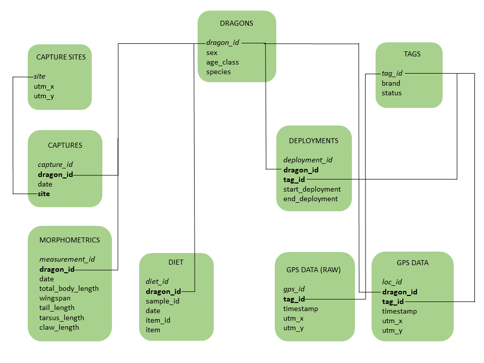
Figure 5.1: Diagram of the dragons database

The database is composed of 9 tables. The dragons table includes individual information on the sample individuals. The captures table contains information on when and where each dragon was captured, and it’s linked to the capture sites table which stores the coordinates of each capture site. The morphometrics table contains body measurements and the diet table contains information on diet samples. Both of these are linked to the dragons table based on individual IDs. We also tracked some of these dragons, so we have a tags table which lists all the different GPS units we deployed within the project. The deployments table tells us which dragon was wearing each tag at any given time, and therefore it’s linked to both the dragons and the tags table through the dragon IDs and the tag IDs, respectively. A raw GPS data table contains telemetry data in its raw form, i.e., as it comes out of the tags, and it’s therefore linked to the tags table via the tag ID. Finally, a processed GPS data table associates the tracking data to the dragons. Primary keys are in italics and foreign keys are in bold. Connectors link tables with one another based on their foreign keys.