Chapter 8 Dynamic Documents with RMarkdown

8.1 What is a dynamic document?

This Chapter is an introduction to creating dynamic documents in R using the rmarkdown package. But what do I mean by dynamic document? In this context, a dynamic document is a file that combines code, the output of that code, and narrative writing all in one. As a matter of fact, you are reading a dynamic document right now: this whole book is written in RMarkdown!

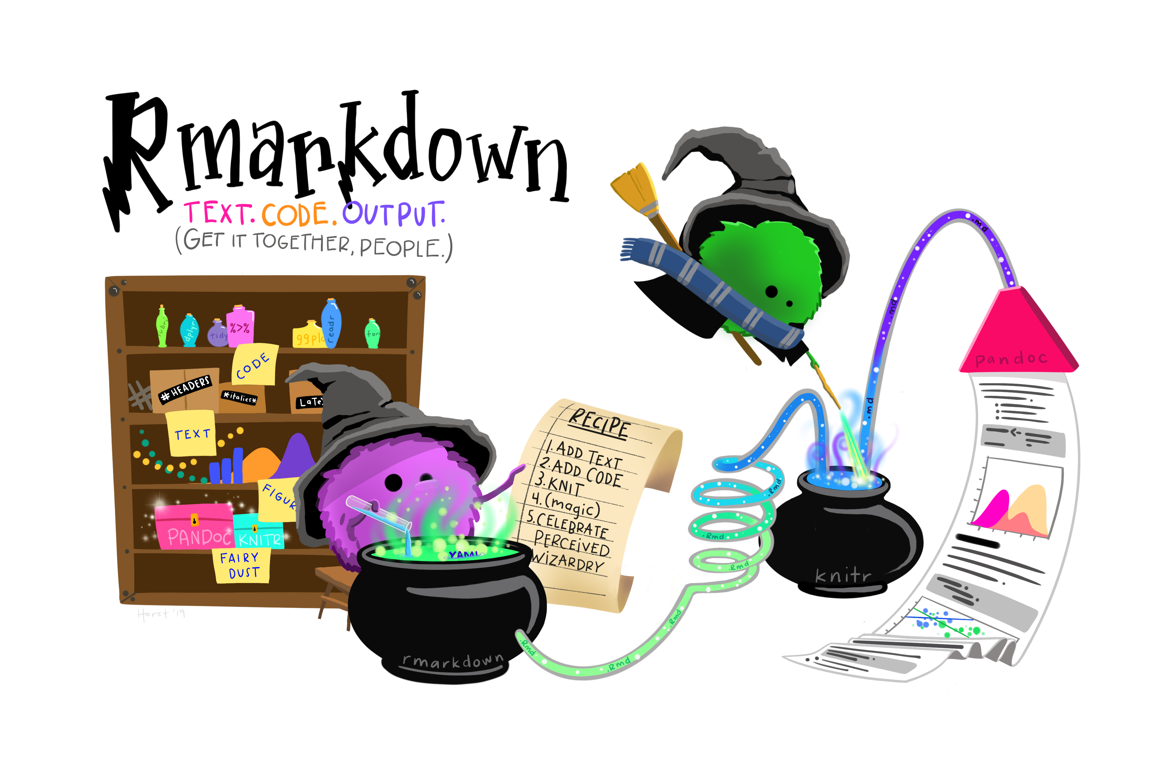
Figure 8.1: Artwork by Allison Horst

In a dynamic document, the code is executed within the document in real time and it produces “living” figures, tables, models, etc. that are updated any time the code itself or the underlying data is updated. We can combine text and code to reproduce any graphical output we want to display in our finished document without having to do anything manually, and the document gets automatically updated any time there is a change upstream in the code or the input data. Because of this, dynamic documents are also reproducible.

8.2 Markdown and RMarkdown

Markdown is a system that translates plain text into HTML (the standard language for creating web pages). RMarkdown is a variant of Markdown specifically created for R that combines Markdown with code and allows you to export dynamic documents in a variety of formats ranging from PDF documents to presentation slides to web pages. The advantages of preparing documents in RMarkdown are numerous:

1. Your text and code are consolidated in the same place rather than in separate documents;
2. You don’t need to save code-generated images and then insert them into a different document;
3. You don’t have to re-save all your plots and manually replace them if you change something in the data or the code;
4. You can forget about all the headaches of having to figure out page breaks or figure placement;
5. You can put all your documents under version control, not just your code.

The file format for RMarkdown is .Rmd. This is the format of the dynamic document that includes code chunks and narrative text. The process of exporting this document into a publishable format (such as .pdf, .html, etc.) is called knitting. The knitting consists of two steps that happen under the hood. First, the R package knitr will take the .Rmd file, run the R code that is contained in it, and convert it into an .md file. The .md file is then passed on to Pandoc, which is a universal document converter. Pandoc will handle the conversion to the final file format.

8.3 Installing RMarkdown

To get started with RMarkdown documents, we need to make sure we have the necessary R packages installed:

install.packages("rmarkdown") 
install.packages("knitr")

8.4 Writing an RMarkdown document

8.4.1 Creating the document

In RStudio, we create a new RMarkdown document by clicking on the File tab and selecting New File > R Markdown.

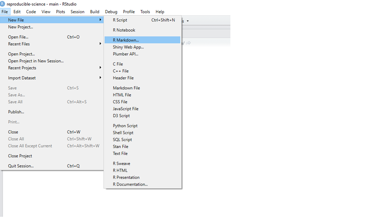
Figure 8.2: Create a new RMarkdown file

A window will pop up asking us what do we want the default format of our document to be. If you are putting together a document to be displayed as a web page, you will select HTML. Even if you want to produce a PDF or other type of document, it’s still a good idea to select HTML here, because you can easily switch from HTML to PDF or others but not the other way around.

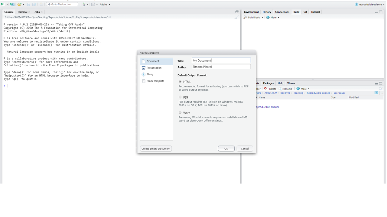
Figure 8.3: Create a new RMarkdown file

8.4.2 YAML headers

Once you click OK, RStudio will create a new document that automatically contains a YAML header. YAML stands for “YAML Ain’t Markup Language” and it encodes the metadata of the document. This is what it looks like:

---
title: "Untitled"
author: "Simona Picardi"
date: "2/18/2021"
output: html_document
---

The author and date were automatically added in, as well as the default output format (HTML). We can go ahead and edit the title, or anything else that is in quotes if we want the date to be different our our name to appear differently (or add more names). The content of the YAML header will appear on top of our document.

8.4.3 Code chunks

Under the YAML header, the template document contains what is called a code chunk:

```{r setup, include=FALSE}
knitr::opts_chunk$set(echo = TRUE)
```

A code chunk is recognized by RMarkdown as containing code. Inside the curly brackets, we specify the language the code is written in (RStudio defaults to R, but we can change this to a different programming language – RMarkdown understands SQL, python, css, and many others.) Then comes the name of the code chunk. This one was automatically named “setup” by RStudio, but we can give it any other name. The important thing is that we can never repeat the same name for a code chunk within the same document. After the comma we can include options that will determine how the code chunk behaves. In this case, the code chunk has the option include=FALSE, which means neither the code or its result will be displayed in the finished document. Other frequently used TRUE/FALSE options are:

• eval: when set to FALSE, the code will not be run when knitting the document (default is TRUE);
• echo: when set to FALSE, the code will not show up in the document but it will be run under the hood and its results will be displayed (default is TRUE);
• warning: this option controls whether warning messages are displayed (default is TRUE);
• error: this option controls whether error messages are displayed (default is FALSE).

By playing with eval and echo we can control whether our code is run and displayed or any combination of these. For example, eval = FALSE, echo = TRUE means our code chunk won’t be run but it will show up in the document (this is great for a tutorial where you want to show someone how to install a package, but you don’t want to reinstall it yourself every time you knit the document); eval = TRUE, echo = TRUE means our code chunk will be displayed as well as run, and its results will be displayed too (this is great for teaching purposes, when you want to show how to write code to produce a certain result); eval = TRUE, echo = FALSE means the code will be run but it will not be visible in the final document (this is great for including a graph in the final document, where the code that produced the graph is not the point.)

To insert a new code chunk in your document, you can click on the green “+C” in your RStudio script toolbar (ore use the shortcut Ctrl + Alt + I).

8.4.4 Inline code

Besides code chunks, you can also embed code within the text using the syntax `r my_code`. The code will be run and the results displayed in its place. For example, if I want to know what 2 + 2 is, I can type `r 2 + 2` in the document and the results displayed will be 4.

To quote code verbatim (which means without interpreting it or executing it, just displaying it), omit the “r” between the two grave symbols. I also like to use the same syntax whenever I mention R functions or any other R-specific words, so it looks like this: function. That makes it clear to the reader that I’m using the word to refer to something that exists in R (a function, an object, a package) and not to the common meaning of that word.

8.4.5 Text formatting

Anything that is not inside a code chunk or inline code is interpreted by RMarkdown as text. There are many different formatting styles that you can achieve with RMarkdown syntax. You can use italics by wrapping text in asterisks, bold with double asterisks, and strikethrough with double tilde. You can add block quotes using a > at the beginning of a line:

This is a block quote.

Or equations:

\[E = mc^{2}\]

The headers in this book are formatted using RMarkdown, and so are bullet lists. Headers are lines that start with one or more hashtags, with the number of hashtags determining the size of the header (one hashtags for main headers, two for sections, three for subsections, etc.) For an overview of how to format text I recommend consulting the RMarkdown cheatsheet. Wonder how I just embedded that link? Just type the words you want to hyperlink in brackets followed by the link in parentheses: []().

8.4.6 Embedding images

Sometimes you may want to add an image in an RMarkdown document that is not code-generated (for example, a photo). There are several ways to do that. One is to use the syntax ![Caption](path_to_image.png) (this needs to be in a new line). Another option is to use the include_graphics function from knitr. You can create a new code chunk where you want the image to appear:

```{r image, fig.cap="this is a caption", fig.align='center', out.width='100%'}
knitr::include_graphics("img/my_image.png")
```

Note the chunk options: fig.cap allows you to add a caption under the figure, fig.align allows you to tweak the alignment of the image with respect to the page, and you can control the size with out.width.

8.4.7 Adding a table of contents

You can add a table of contents to your document by adding an option for it in the YAML header:

---
title: "Untitled"
author: "Simona Picardi"
date: "2/18/2021"
output: 
  html_document:
    toc: true
    toc_depth: 2
---

The option toc: true activates the table of contents. You can then list additional options to tweak the appearance of the table of contents. For example, toc_depth controls how many header levels are visible in the table of contents (default is 3, which means headers that range from #-###). Another option is toc_float, which means the table of content will float on the side of the page even as we scroll down.

8.4.8 Knitting the document

When you are done composing your document and you want to see the rendered version, it’s time to knit. You can click Knit on the RStudio script toolbar and the process will start.

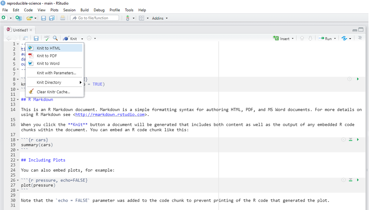
Figure 8.4: Knitting an RMarkdown file

You will see the progress status in the console. If there are any formatting mistakes, you will get an error that points you to the line where the problem is. A very common reason why knitting may fail is if you forgot to give the code chunks different names, so watch out for that! Once the knitting is complete, you’ll find an HTML file in your working directory with the same name as the .Rmd file. Double click on it, and your rendered document will open in a browser window.

8.4.9 The sky is the limit!

This is a brief overview on how to get started with RMarkdown, but the sky is the limit when it comes to possibilities for customization of RMarkdown documents. You can add tables, footnotes, and even a bibliography to your document which can be automatically synchronized with your reference management system. You can choose among several different themes for your rendered document or you could even make your own theme. Here are some great resources if you want to learn more about these and other functionalities of RMarkdown:

• The RStudio tutorial to RMarkdown
• R Markdown: The Definitive Guide
• Creating Dynamic Documents with RMarkdown and Knitr